$$ \require{color} \require{newcommand} \definecolor{myblue}{RGB}{ 31,120,180 } \definecolor{mygreen}{RGB}{ 51,160,44 } \definecolor{myred}{RGB}{ 227,26,28 } \definecolor{myorange}{RGB}{ 255,127,0 } \definecolor{mypurple}{RGB}{ 106,61,154 } \def\xa{ {\color{myblue} x_1} } \def\xb{ {\color{mygreen} x_2} } \def\xc{ {\color{myorange} x_3} } \def\yy{ {\color{mypurple} y} } $$

Introduction

In this writeup, I will go over some visualisations I made to help me better understand some rudimentary mathematical concepts from the course of Convex Optimisation by Stephen Boyd. I have attempted to use optical illusions, also known as 3D plots, to try to visualise these sets in a bit more detail than possible in Flatland.

The introduction in the book explains how to create affine, convex and conic sets using linear combinations. All the aforementioned sets are expressed as a linear combination of some seed vectors $x_i$ in $\mathbb{R}^n$ using scalar coefficients $\theta$ in $\mathbb{R}$.

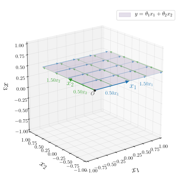
The general form of the generator equation for these sets is $$\yy=\theta_1 \xa + \theta_2 \xb + \ldots + \theta_n x_n$$

A set is thus constructed by plugging in all possible $\theta_i$'s to obtain all possible $\yy$'s. The way in which the sets discussed will differ, is in the values we allow the $\theta_i$'s to take on. Constraints on the coefficients $\theta_i$ we will work with are:

Constraint on $\theta_i$	Equation	Symbol
Sum to 1	$\sum_{i}\theta_i = 1$
Non-negative	$\theta_i \geq 0 \quad \forall i$

We shall refer to these constraints using the symbols in the last column, which are hopefully intuitive. For all visualisations below, the $x_i$'s will be in $\mathbb{R}^3$. I will use unit vectors for $\xa$, $\xb$ and $\xc$, but the same plots could have been drawn for arbitrary vectors.

Affine sets

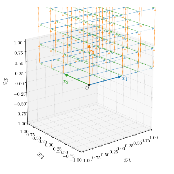
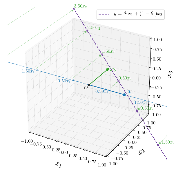
As hinted by the symbol following the title, we get affine sets if we only impose that $\theta_i$'s sum to $1$. If we have two vectors $\xa, \xb$ in $\mathbb{R}^3, \xa \ne \xb$, then for any scalar values $\theta_i$ \begin{align} \yy&=\theta_1 \xa + \theta_2 \xb, \quad \text{where} \quad \theta_1 + \theta_2 = 1 \\ &=\theta_1 \xa + (1 - \theta_1) \xb \end{align}

$\yy$ will be in the affine set, the line that passes through the head of vectors $\xa$ and $\xb$. The points $\yy$ can be generated by scaling vector $\xa$ by $\theta_1$ and then adding that vector to the result of scaling $\xb$ by $(1-\theta_1)$. This combination of vectors is visualised using dotted vectors below.

However, while this visual construction shows how the points created when choosing $\theta_1$ in such a way lie on a line, the result is more complex than it needs to be. This is so since we are still bestowing upon $\theta_2 = 1 - \theta_1$ and $\theta_1$ the priviledge of free parameters, when in reality $\theta_2$ is powerless, there is only one free parameter because of the constraint.

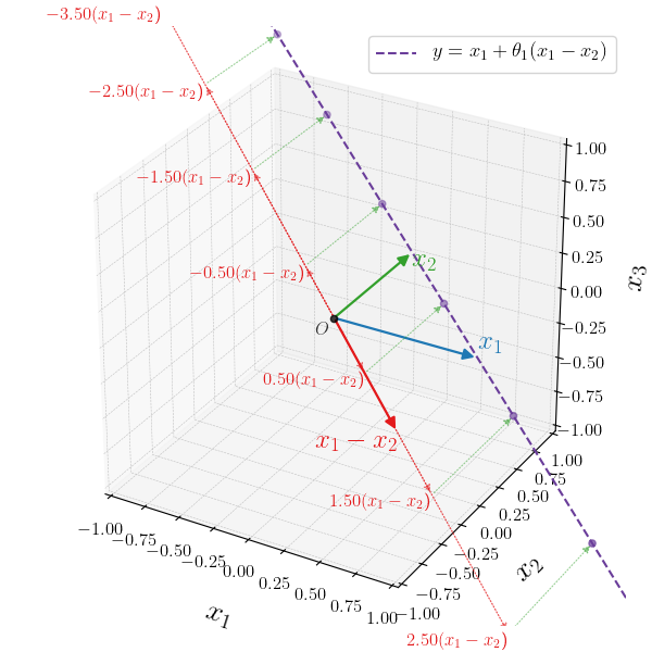
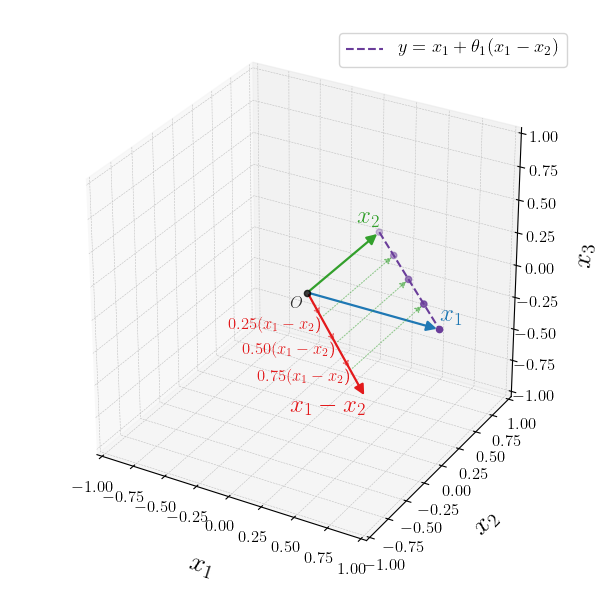
A clearer way to see the affine set, is to regroup the terms containing $\theta_1$.

\begin{align} \yy &=\theta_1 \xa + (1 - \theta_1) \xb \\ & =\theta_1 \xa + \xb - \theta_1\xb \\ & =\xb + \theta_1 (\xa - \xb) \end{align}

After this algebraic manipulation, we get a much clearer visual understanding of the situation. We compute the vector $\xa - \xb$, which we scale using all possible values of $\theta_1$. We then offset the result by $\xb$ to get all possible points on the line, the affine set.

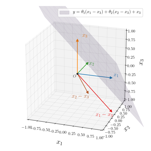
In the case where we have 3 non collinear vectors, the situation generalizes as follows:

\begin{align} \yy &=\theta_1 \xa + \theta_2 \xb + (1 - \theta_1 - \theta_2) \xc \\ &=\theta_1 \xa + \theta_2 \xb + \xc - \theta_1 \xc - \theta_2 \xc \\ &=\theta_1 (\xa - \xc) + \theta_2 (\xb - \xc) + \xc \end{align}

This time we calculate two differences, $\xa - \xc$ and $\xb - \xc$. We notice that taking all linear combinations of these vectors, $\theta_1 (\xa - \xc) + \theta_2 (\xb - \xc)$ fill the semi-transparent brownish plane.

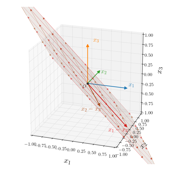
Now, if we offset this plane by $\xc$, we generate our target affine set. Something that is clearer from the plot than the equations, is that we could actually offset the plane by any of the vectors $\xa$, $\xb$ or $\xc$ and still get the target affine set. Depending on which vector is used, each point from the brownish plane through the origin $O$ will get offset to a different point on the plane. However, the plane has infinite points, so the difference would be indistinguishable.

Convex sets

For convex sets, we can continue from where we left off with the affine set. $$\yy=\xb + \theta_1 (\xa - \xb)$$ However, for a convex set we further constrain the thetas to be positive. Constraining $\theta_1$ to be positive, limits the range of vectors we can produce when scaling $\xa - \xb$ by $\theta_1$, as can be seen in the plot below. This means, the vectors in our set lie on a line segment joining $\xb$ and $\xa$.

In the 3D case: $$\yy=\theta_1 (\xa - \xc) + \theta_2 (\xb - \xc) + \xc$$ we are constrained to a 2-simplex (triangle).

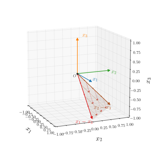
As before, we can add the offset $\xc$. Note, however, that in this case we can only offset by $\xc$ if we want to get the target convex set.

Conic sets

For Conic sets we only have the constraint that $\theta_i$'s should be positive. So for the 2D case: $$\yy=\theta_1 \xa + \theta_2 \xb, \quad \theta_1,\theta_2 \geq 0$$ our two parameters, $\theta_1$ and $\theta_2$, are not entangled through some constraint, but are both required to take values in the positive quadrant of $\mathbb{R}^2$. Therefore, we can only combine our seed vectors $\xa$ and $\xb$ to get $\yy$ in ways that "remain between" the two vectors.

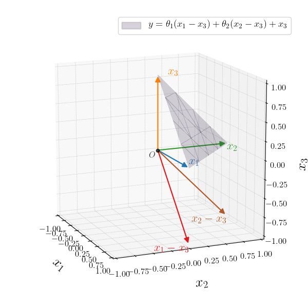
For the 3D case

$$\yy=\theta_1 \xa + \theta_2 \xb + \theta_3 \xc, \quad \theta_1,\theta_2, \theta_3 \geq 0$$

we can offset the current set using $\xc$ scaled by positive values of $\theta_3$.